A Market of Many Markets

The question

Where should a market analyst look closer?

In a real estate investment scenario, I explored which economic, housing, demographic, and geographic characteristics are associated with higher median housing values. The aim is to support local market research and identify where additional investigation is needed.

The data

An area-level view of California.

The scikit-learn California Housing dataset contains 20,640 observations and eight predictors: median income, house age, average rooms, average bedrooms, population, average occupancy, latitude, and longitude. The target is median house value in $100,000 units.

No missing values or duplicate rows were identified. Observations represent areas rather than individual properties; the target clusters at an upper cap of approximately $500,000.

The approach

Explore the market. Establish a baseline.

• Review distributions and the correlation matrix; examine income against value and map geographic patterns.
• Split 80% training and 20% test data using random_state=42.
• Fit Linear Regression with all eight predictors. Keep target values in original $100,000 units.
• Report test R² and RMSE, converting RMSE to dollars for interpretation.

The evidence

Income matters. So does location.

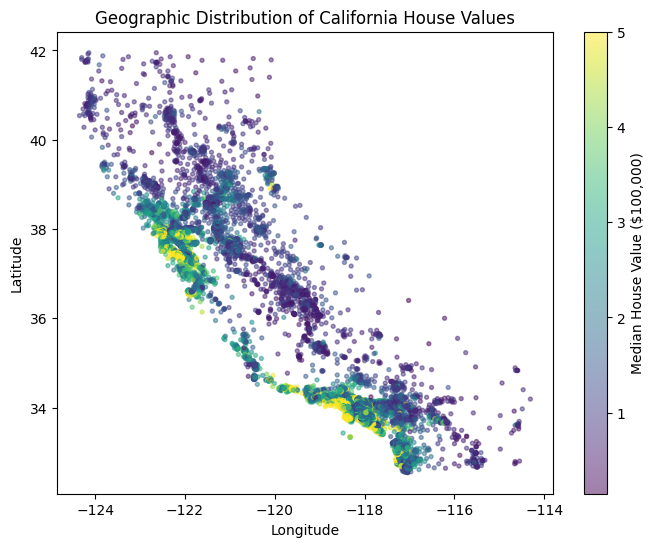
Median income has the strongest positive direct correlation with median house value (r = 0.69). Average rooms (r = 0.15) and house age (r = 0.11) have weaker positive relationships. Geographic clusters show why similar housing attributes can accompany different area values.

The eight-predictor model explains about 58% of held-out variation. RMSE gives more weight to larger errors; it is not the mean absolute error or an error bound for every area.

The business recommendation

Research locally. Combine economic and geographic context.

Use income and location together to prioritize areas for deeper research. Treat the regression as a baseline for decision support, then incorporate current local information before evaluating opportunities.

This case demonstrates market analysis and a predictive baseline. It does not measure investment returns or produce individual-property appraisals.

What I would improve

The baseline is only the beginning.

• Area-level estimates do not describe the condition or market value of an individual home.
• The target cap limits interpretation in higher-value areas. This is benchmark data rather than a current market feed.
• A random split does not establish performance in entirely new regions or future periods. Geographic validation would be a useful next step.
• Additional local context, such as amenities, employment access, and property characteristics, could support a stronger future model.

Sources & code

Go a layer deeper.

Python · pandas · NumPy · scikit-learn · Matplotlib · seaborn

The business narrative comes from the supplied presentation; model setup and results were cross-checked against the supplied notebook and its saved outputs. Presentation downloads are optimized visual copies. Original data files are required to rerun the analyses.